Applying Machine Learning and LSTM for Classifying EEG Signals

Figuring out a way to make movement possible for patients who have lost limbs due to amputation or neurological disability is an urgent goal of the global medical community. But before movement of a prosthetic or paralyzed limb can be achieved, it is necessary to come up with a valid method for classifying brain signals for brain-computer interface.

The brain-computer interface is a pathway created for the exchange of information between the brain and a digital device for controlling a patient’s motor function. Establishing this pathway of brain-computer communication is a crucial step in making it possible for disabled patients to move again.

Azoft R&D team, together with Sergey Alyamkin and Expasoft, decided to research the topic of building a brain-computer interface and participated in “Grasp-and-Lift EEG Detection” competition organized by Kaggle. According to competition rules, participants were given 2 months to identify with the lowest probability of error and classify various movements of the right hand using EEG (electroencephalogram), which is a recording of the electrical activity of the brain.

To achieve this goal, we had to create a model that would allow us to classify movements of the right hand based on data gathered using EEG. Work on the model consisted of several stages: studying the biological aspects of the project, preprocessing of data, feature extraction of a signal and choosing the most appropriate machine learning algorithms.

Biological Aspects of the Project

Having spent some time studying the basics of brain structure and function, we were able to come up with the following conclusions.

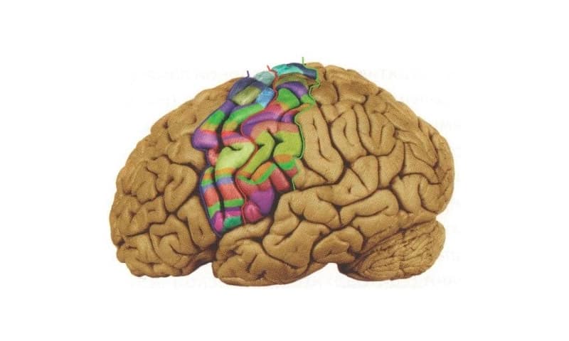
• First, the cerebral cortex plays a leading role in the mental processes of the human brain.
• Second, there are several areas of the brain, responsible for various motor and sensory functions.

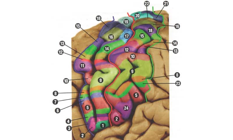
As shown in the image above, the sensorimotor centers of the human brain are: 1) root of the tongue; 2) larynx; 3) palate; 4) lower jaw; 5) tongue; 6) lower part of the face; 7) upper part of the face; 8) neck; 9) fingers; 10) hand; 11) arm from shoulder to wrist; 12) shoulder; 13) shoulder blade; 14) chest; 15) abdomen; 16) lower leg; 17) knee; 18) thigh; 19) toes; 20) the big toe; 21) four toes; 22) foot; 23) face; 24) pharynx. As shown in the image above, the motor area of the cortex is located between the blue and red lines, whereas the sensorimotor area is between the red and green lines.

Finally, we learned that the main brain activity associated with hand movement is in the range from 7 to 30 Hz.

Data Preprocessing

The next step our team had to take was data preprocessing, during which we carried out filtering and downsampling of the data. The main objects of the study in the EEG signal were eye movement, the movement of the electrodes, the contraction of muscles of the head and the heart, and network interference 50-60 Hz. Interference caused by movement of eyes, muscles, and electrodes, are arranged at lower frequencies (from 0.1 Hz to 6 Hz), compared to useful signals. Therefore, we decided to use a bandpass filter with bandwidth of 7 to 30 Hz. It is important to note that the digital filtering contributed the least distortion in the signal, so we chose a filter with finite impulse response.

As for decimation, which is the process of reducing the sampling rate of a signal, we dropped it from 500 to 62.5 Hz. Since the maximum useful frequency is 30 Hz, taking into consideration the Nyquist theorem, the sampling rate must be greater than 60 Hz.

Identification of Brain Signal Appearance

We used several different approaches to identify typical signs of brain signals. This was necessary in order to reduce the amount input data, exclude redundant information, and increase accuracy of brain signal classification. The testing methods included principal component analysis, electrode selection from the biological view point, and wavelet transform.

Eventually, we had to stop using principal component analysis. It was assumed that deep brain signals are mutually orthogonal in calculating compulsory matrix by means of SVD — singular value decomposition. In practice, it turned out that they were not mutually orthogonal. Besides, in the experiment we had 32 detectors, which is not enough for good SVD. It would be better to use ICA (independent component analysis) for nonorthogonal signals. Unfortunately, we ran out of time and didn’t try ICA.

When choosing electrodes, our decision was based on their spatial arrangement. In the following picture, the electrodes that provided data are labeled with the numbers from 1 to 32.

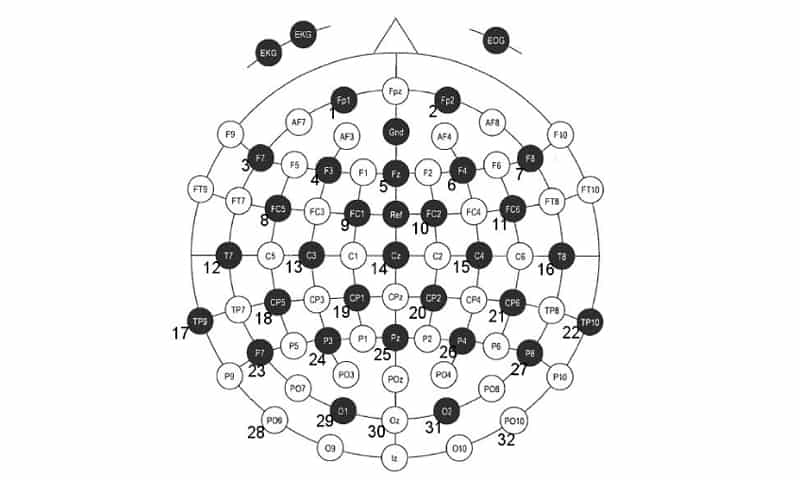
Having chosen the required electrodes, we decided to focus on wavelet transform as our key method of brain signal identification. There is an implied principle of wavelet choice: the basic wavelet-function’s look has to be similar to the typical manipulated signal. Using this approach, we can analyze the fine structure of signals by means of their simultaneous localization based on both frequency and time.

Choosing a Machine Learning Algorithm

When choosing the best machine learning algorithm for the task, we decided to apply the familiar convolutional neural networks (CNN), which are a part of deep learning algorithms. Сonvolutional neural networks are among the most commonly used neural network types, especially for tasks that involve two-dimensional signals (i.e. images). Although, these networks can also work with regular signals.

Thanks to a convolutional neural network, we identified that 4096 samples(up to downsampling) yield the least error rate in the final model. The derived model enabled us to calculate the area under ROC curve, which equals 0.91983.

The second experimental algorithm was the so-called “random forest” since it is one of the most popular methods for classification today. This algorithm consists of a set of decisions trees, each of them gets its own dataset from the total dataset. We ran out of time trying a combination of “wavelet transform + random forest” because wavelet transform is very time-consuming

The third chosen machine learning algorithm was RNN (recurrent neural networks). One of the main characteristics of RNN is back coupling. Biological neural networks are recurrent. They have memory, which allows to not convey signal history to the network.

We ran multiple experiments with the recurrent neural network, tested various architectures and back coupling delay. The network didn’t learn. There was a problem with memory — we could not create a complex network with more than two layers. Then we came to the conclusion that we need to try a special type of neural networks — LSTM (long short term memory). Nonetheless, the complexity of the LSTM algorithm requires deeper investigation than it was possible under the competition circumstances. For these reasons, we decided to stop at the current stage, without obtaining LSTM testing results.

The Outcome

Finally, our R&D team was able to obtain a high-quality classification of EEG signals during the process of hand movements. Thanks to the quality parameter “area under ROC curve”, which was derived as a result of using convolutional neural networks, we verified that deep learning algorithms are effective in various types of signal classification. Therefore, we can conclude that CNN and fully convolutional networks are one of the greatest deep learning methods for the development of a brain-computer interface. In simple words, show us your EEG signals and we’ll figure out what you were doing at the moment of EEG recording.