Applied Use of M2M Communication: Traffic Sign Recognition in iOS Apps

The future of mobile industry, and software industry as a whole, is becoming more and more intertwined with the applied use of M2M technologies. The latest advances in M2M make it possible to develop innovative, more efficient solutions in various business spheres: business automation, security and CCTV monitoring, consumer electronics, health care, etc.

Apple Inc. recently made its first step in the M2M direction, having announced the forthcoming release of ‘iOS in the car’ — a mobile platform that allows to integrate iOS devices with a car in-dash system. It’s time for us iOS developers get started as well.

Our team’s current project is developing an iOS app prototype to assist the driver in traffic sign recognition. The app turns an iOS device into a dashboard camera that records the traffic and recognizes road signs. This allows the driver to quickly check what the last sign was, in case he/she missed it or simply forgot (for example, forgot what the speed limit is for a given road).

Project overview

The main concept of the project is to expand iOS device abilities and turn it into the driver’s assistant (i.e. co-pilot). The task at hand is to develop a prototype app that not just records what’s happening on the road but also warns the driver and is capable of road sign ricognition.

When working on sign-recognition functionality, we limited it only to regulatory signs that are round-shaped signs with a white background and a red border. In the future, we plan to add the rest of sign types and implement a constantly updated database containing information about various roads and traffic signs, accessible to all devices with the app installed.

Note: Some traffic signs in North America are quite different European signs. Our prototype was developed according to European traffic signs. In the future, we are planning to expand the functionality to American signs as well.

Here’s how the app works: the iPad/iPhone cam records a video stream in resolution 1920×1080, the app analyzes the received frames, detects signs and associate them with signs in a database. When a sign has been recognized, some event is launched: to warn a driver, to add new data to the database, etc.

The task falls into two stages:

• Color-based image segmentation
• Sign recognition

Stage 1. Color-Based Image Segmentation

Image capturing. Detection of red and blue colors

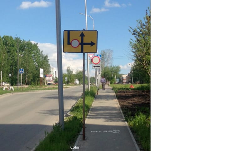
Most regulatory signs are round with a red border and a white background. Keeping this in mind, we’ll try to develop an algorithm for recognizing such signs in an image. We’re going to work with a freshly captured RGB image. To begin, we have to crop the image into a square of 512×512 pixels (fig. 1) and extract red and white colors while ignoring the others. The problem here is that RGB is not the most convenient color model for localizing colored areas. Red is rarely found in the world as a pure color. It is almost always mixed with other primary colors. The colors also have varying brightness and hue depending on the lighting. For example, many things appear tinted slightly red at dusk and dawn. Twilight also affects the color in a different way.

At first, we tried to process the image in RGB. To extract red areas we used threshold values of R > 0.7, G < 0.2, B < 0.2. However, this approach turned out to be suboptimal, because the colors are highly dependent on the time of day and lighting conditions. The same color has different channel values on a sunny and on a cloudy day.

These problems can be avoided by using the HSV/B color model that represents colors as combination of attributes hue, saturation, and value/brightness. This model is often pictured as a cylinder.

In the HSV/B model shades of color become illumination-invariant, simplifying the task of color extraction regardless of the weather and light conditions (time, weather, shadows, sun, etc.). The conversion from RGB to HSV/B is performed by the shader below:

varying highp vec2 textureCoordinate; 
precision highp float; 
 
uniform sampler2D Source; 
 
void main() 
{ 
 vec4 RGB = texture2D(Source, textureCoordinate); 
 
 vec3 HSV = vec3(0); 
 float M = min(RGB.r, min(RGB.g, RGB.b)); 
 HSV.z = max(RGB.r, max(RGB.g, RGB.b)); 
 float C = HSV.z - M; 
 if (C != 0.0) 
 { 
 HSV.y = C / HSV.z; 
 vec3 D = vec3((((HSV.z - RGB) / 6.0) + (C / 2.0)) / C); 
 if (RGB.r == HSV.z) 
 HSV.x = D.b - D.g; 
 else if (RGB.g == HSV.z) 
 HSV.x = (1.0/3.0) + D.r - D.b; 
 else if (RGB.b == HSV.z) 
 HSV.x = (2.0/3.0) + D.g - D.r; 
 if ( HSV.x < 0.0 ) { HSV.x += 1.0; } 
 if ( HSV.x > 1.0 ) { HSV.x -= 1.0; } 
 } 
 
 gl_FragColor = vec4(HSV, 1); 
}

To extract red areas of the image we’re going to build 3 intersecting planes that form a region within the HSV/B cylinder which corresponds to the red color range. Extracting white is easier because it’s located in the central part of the cylinder, so we can just specify the range for white in threshold values for point distance (S axis) and height (V axis) in the cylindrical coordinates. The shader code for this procedure is below:

varying highp vec2 textureCoordinate; 
precision highp float; 
 
uniform sampler2D Source; 
 
//parameters that define plane 
const float v12_1 = 0.7500; 
const float s21_1 = 0.2800; 
const float sv_1 = -0.3700; 
 
const float v12_2 = 0.1400; 
const float s21_2 = 0.6000; 
const float sv_2 = -0.2060; 
 
const float v12_w1 = -0.6; 
const float s21_w1 = 0.07; 
const float sv_w1 = 0.0260; 
 
const float v12_w2 = -0.3; 
const float s21_w2 = 0.0900; 
const float sv_w2 = -0.0090; 
 
void main() 
{ 
 vec4 valueHSV = texture2D(Source, textureCoordinate); 
 
 float H = valueHSV.r; 
 float S = valueHSV.g; 
 float V = valueHSV.b; 
 
 bool fR=(((H>=0.75 && -0.81*H-0.225*S+0.8325 <= 0.0) || (H <= 0.045 && -0.81*H+0.045*V-0.0045 >= 0.0)) && (v12_1*S + s21_1*V + sv_1 >= 0.0 && v12_2*S + s21_2*V + sv_2 >= 0.0)); 
 float R = float(fR); 
 float B = float(!fR && v12_w1*S + s21_w1*V + sv_w1 >= 0.0 && v12_w2*S + s21_w2*V + sv_w2 >= 0.0); 
 
 gl_FragColor = vec4(R, 0.0, B, 1.0); 
}

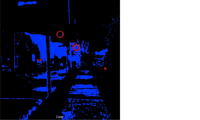
An example output of the color extraction shader is presented on fig. 2. The image resolution here is 512×512, but we’re going to continue working with the image downsampled to 256×256. Tests have shown that 256×256 resolution gives a significant performance boost and the quality is still good enough for sign recognition.

Circle detection

The majority of circle detection methods work with binary images. The red-white image that’s been acquired in the previous step has to be converted into binary for further processing. In this project we assume that regulatory traffic signs consist of a white circle with a red border, so we developed a shader algorithm that looks for this kind of edges in a red-white image, marking edge pixels as 1 and the rest as 0. The algorithm works as follows: for every red pixel in the input image, neighboring pixels are checked for white; if at least one white pixel is found, the red pixel is marked as an edge pixel.

The resulting image is a 256×256 pixel bitmap with a black background and white pixels designating the detected edges. In order to reduce noise, morphological noise removal algorithm is applied.

The next step is to detect circles in the binary image. Originally we tried to do this using the OpenCV CPU implementation of the Hough Circle Transform method. Unfortunately, tests have shown that this approach results in a very high CPU load and an unacceptable performance level. While a reasonable solution to this problem could be porting the algorithm to GPU shaders, many circle detection methods including the Hough transform are not completely suitable for running inside a shader. Therefore, we had to use a slightly more exotic method called Fast Circle Detection Using Gradient Pair Vectors, that provides substantial CPU performance increase. In a nutshell, this method has the following steps:

1. A gradient direction vector is calculated for every pixel of the binary image. The vector represents brightness gradient direction and it’s calculated using Sobel operator implemented in the following shader:

varying highp vec2 textureCoordinate; 
precision highp float; 
 
uniform sampler2D Source; 
uniform float Offset; 
 
void main() 
{ 
 vec4 center = texture2D(Source, textureCoordinate); 
 
 vec4 NE = texture2D(Source, textureCoordinate + vec2(Offset, Offset)); 
 vec4 SW = texture2D(Source, textureCoordinate + vec2(-Offset, -Offset)); 
 vec4 NW = texture2D(Source, textureCoordinate + vec2(-Offset, Offset)); 
 vec4 SE = texture2D(Source, textureCoordinate + vec2(Offset, -Offset)); 
 vec4 S = texture2D(Source, textureCoordinate + vec2(0, -Offset)); 
 vec4 N = texture2D(Source, textureCoordinate + vec2(0, Offset)); 
 vec4 E = texture2D(Source, textureCoordinate + vec2(Offset, 0)); 
 vec4 W = texture2D(Source, textureCoordinate + vec2(-Offset, 0)); 
 
 vec2 gradient; 
 gradient.x = NE.r + 2.0*E.r + SE.r - NW.r - 2.0*W.r - SW.r; 
 gradient.y = SW.r + 2.0*S.r + SE.r - NW.r - 2.0*N.r - NE.r; 
 
 float gradMagnitude = length(gradient); 
 float gradX = (gradient.x+4.0)/255.0; 
 float gradY = (gradient.y+4.0)/255.0; 
 
 gl_FragColor = vec4(gradMagnitude, gradX, gradY, 1.0); 
}

2. The non-zero vectors are grouped by directions. There are 48 directions in total due to input image discretization or 48 groups.

3. Every group is searched for a pair of vectors V1 and V2 that are in opposite directions (e.g. 45 and 225 degrees). The pairs are checked to satisfy the following conditions: the angle beta should be less than a given threshold; the distance between P1 and P2 should be less than the maximum diameter of a circle and greater than the minimum diameter. If the conditions are met, the midpoint C that divides the line segment P1P2 in half is assumed to be the center of the circle. Next, C is placed in a so-called accumulator. The accumulator is a 3-dimensional array of size 256x256x80. The first 2 dimensions (256×256 is the size of the input image) correspond to centers of circles. The third dimension (80) corresponds to the radius of the circle with a maximum radius of 80. Thus, a response for every gradient pair is accumulated in a point that matches a circle of some radius.

4. The accumulator is then scanned for centers where at least 4 vector pairs with different directions have been found (e.g. pairs of vectors 0 and 180, 45 and 225, 90 and 270, 135 and 315). Closely located centers are merged into one. In case circles of different radiuses are found in the same point, they’re also merged into one with the maximum radius.

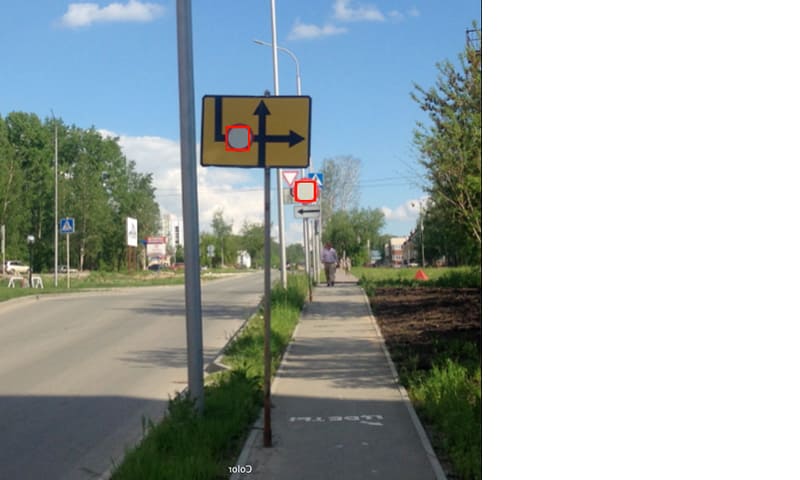
Stage 2. Localized sign recognition

Localized circles that are supposed to contain regulatory signs are cut out and scaled to a common size of 28×28 pixels. The resulting images are processed with Sobel operator and passed to a convolutional neural network pre-trained on a set of sign images.

We already explained the principles behind neural networks in a post about our credit card numbers recognition system. Our project involved multi-layer convolutional neural networks. Segmented signs are passed down to a convolutional neural network based on an algorithm published by Yann LeCun, Leon Bottou, Yoshua Bengio and Patrick Haffner. The network is trained on a set of sample images.

Recognition algorithm results in a set of probabilities of known sign types for every block of the processed image. Sometimes, it takes several attempts to capture and recognize a sign with a high probability. Unrecognized signs are processed again in the next frame for higher accuracy. A sign is considered to be well recognized if its probability is higher than some predefined threshold.

Conclusion

This co-pilot app prototype is our first M2M project but definitely not the last one. In the near future, we plan to continue our research in this field: recognition for all road sign types, expanding the brightness range by adding special modes for bright daylight, twilight, sunset, etc.

The main challenge with recognizing other road sign types is to detect shapes other than a circle, such as triangles, squares, etc. At the moment, we don’t have an optimal solution, but we’re working on several options that have both advantages and disadvantages. If you have experience with color-based segmentation of triangular and rectangular shapes, we’d really appreciate your comments and feedback!